INVASE: INstance-wise VAriable SElection using neural networks [Literature Survey]
Authors: Jinsung Yoon, James Jordon, Mihaela van der Schaar
Conference: ICLR 2019
Problem Statement: Instance-wise feature selection where there can be different number of features selected for each instance.
Motivation and Methodology: Instance-wise feature selection was introduced by the L2X[2] paper in 2018. It involves finding a subset of features that are most informative for each given example. But, in their methodology, the user had to provide the number of features to be selected as input. This could lead to the problem of over-explanation. So, to mitigate this problem the authors of the INVASE paper take a different approach wherein they try to minimize the KL divergence between the conditional distributions \(Y \vert X\) and \(Y \vert X_S\). And, in order to bypass the pain of backprop through sampling, the authors use an actor-critique framework from the RL literature.
At this point it might not be clear how doing the above solves the issue that we had, but it does and we will see how soon.
Methodology in detail:
 Taken from the INVASE[1] paper
Let \(\mathcal{X}\) be a \(d\)-dimensional feature space,
\[\mathcal{X}=\mathcal{X}_{1} \times \ldots \times \mathcal{X}_{d}\]and \(\mathcal{Y}\) be a discrete label space,
\[\mathcal{Y}=\{1, \ldots, c\}\]Let \(\mathbf{X}=\left(X_{1}, \ldots, X_{d}\right) \in \mathcal{X}\) and \(\mathbf{Y} \in \mathcal{Y}\) be random variables with joint p.m.f.(or p.d.f.) be \(p\) and marginal p.m.f.(or p.d.f.) be \(p_X\) and \(p_Y\) respectively.
Let \(\mathbf{s} \in\{0,1\}^{d}\) be the selection vector, where if \(s_i=1\) that means \(i^{th}\) feature is selected, else if \(s_i=0\) then the \(i^{th}\) is not selected. Let \(∗\) be any point not in any of the spaces \(\mathcal{X_1} , ..., \mathcal{X_d}\) and define \(\mathcal{X}^{*}_{i} = \mathcal{X}_i \cup {∗}\) and \(\mathcal{X}^{∗} = \mathcal{X}^{*}_{1} \times ... \times \mathcal{X}^{*}_{d}\) . Given \(x \in \mathcal{X}\)(\(x\) is an instance of the random variable \(X\)) we will write \(x^{(s)}\) to denote the suppressed feature vector defined by
\[x_{i}^{(\mathbf{s})}=\left\{\begin{array}{l} x_{i} \text { if } s_{i}=1 \\ * \text { if } s_{i}=0 \end{array}\right.\]here, \(*\) represents that the feature is not selected.
Now, this selection vector \(s\) is generated by a selector function \(S:\mathcal{X} \rightarrow \{0,1\}^{d}\), which takes \(x\) as input and returns a \(d\) dimensional binary vector as output.
Objective:
find \(S\) such that \(\left(Y \mid \mathbf{X}^{(S(\mathbf{x}))}=\mathbf{x}^{(S(\mathbf{x}))}\right) \stackrel{d .}{=}(Y \mid \mathbf{X}=\mathbf{x})\)(distributional similarity), and \(S(x)\) is minimal i.e. as few features selected as possible.
Optimization problem:
The loss is a simple representation of the objective via KL divergence between distributions. The loss as a function of the selector function \(S\) is given as: \(\mathcal{L}(S)=\mathbb{E}_{\mathbf{x} \sim p_{X}}\left[K L\left(Y|\mathbf{X}=\mathbf{x} \| Y| \mathbf{X}^{(S(\mathbf{x}))}=\mathbf{x}^{(S(\mathbf{x}))}\right)+\lambda\|S(\mathbf{x})\|\right]\)
where \(\| · \|\) simply denotes the number of non-zero entries of a vector and \(\lambda\) is a hyper-parameter for tradeoff between distributional similarity and number of features being selected.
Let the KL divergence term be denoted as \(l(x,S(x))\) or \(l(x,s)\) and after a bit of simplification, \(l(\mathbf{x}, \mathbf{s})=\int_{\mathcal{Y}} p_{Y}(y \mid \mathbf{x})\left[\log \left(p_{Y}(y \mid \mathbf{x})\right)-\log \left(p_{Y}\left(y \mid \mathbf{x}^{(s)}\right)\right)\right] d y\) So, our loss function can be re-written as: \(\mathcal{L}(S)=\mathbb{E}_{\mathbf{x} \sim p_{X}}[l(\mathbf{x}, S(\mathbf{x}))+\lambda\|S(\mathbf{x})\|]\)
Now, if you notice, our loss function has some distributions( \(p_Y(y\vert\mathbf{x})\) and \(p_Y(y \vert \mathbf{x}^{S(\mathbf(x))})\) ) which we do not know. So, to solve this issue the authors use an actor-critique framework to estimate these distributions.
The authors introduce a pair of functions:
\[\begin{array}{l} f^{\phi}: \mathcal{X}^{*} \times\{0,1\}^{d} \rightarrow[0,1] \\ f^{\gamma}: x \rightarrow[0,1]^{c} \\ f^{\phi} \text { will estimate } p_{Y}\left(\cdot \mid x^{(s(x))}\right)\\ f^{\gamma} \text { will estimate } p_{Y}(\cdot \mid x) \end{array}\]\(f^{\phi}\) is called the predictor network and \(f^{\gamma}\) is called the baseline network. Now by using these two networks, they estimate the KL divergence term( \(l(x,s)\) ) in the original loss equation by \(\hat{l}(x,s)\) which is defined as follows(for fixed \(\phi\) and \(\gamma\)):
\[\hat{l}(\mathbf{x}, \mathbf{s})=-\left[\sum_{i=1}^{c} y_{i} \log \left(f_{i}^{\phi}\left(\mathbf{x}^{(\mathbf{s})}, \mathbf{s}\right)\right)-\sum_{i=1}^{c} y_{i} \log \left(f_{i}^{\gamma}(\mathbf{x})\right)\right]\]Dealing with a large selection space:
Another issue with feature selection problems is the exponentially large selection space. So, to deal with that the selector network induces a probability distribution over the selection space(\(\{0,1\}^{d}\)). The joint probability distribution(or the policy) is given as follows:
\[\pi_{\theta}(x, s)=\prod_{i=1}^{d} \hat{S}_{i}^{\theta}(x)^{s_{i}}\left(1-\hat{S}_{i}^{\theta}(x)\right)^{1-s_i}\]here, \(\hat{S}^{\theta}\) is the neural network used to approximate the selector function. \(\hat{S}_{i}^{\theta}\) represents the probability with which we select the \(i^{th}\) feature.
Finally, the loss of the selector function is defined as follows(with approximations for distributions we donot know):
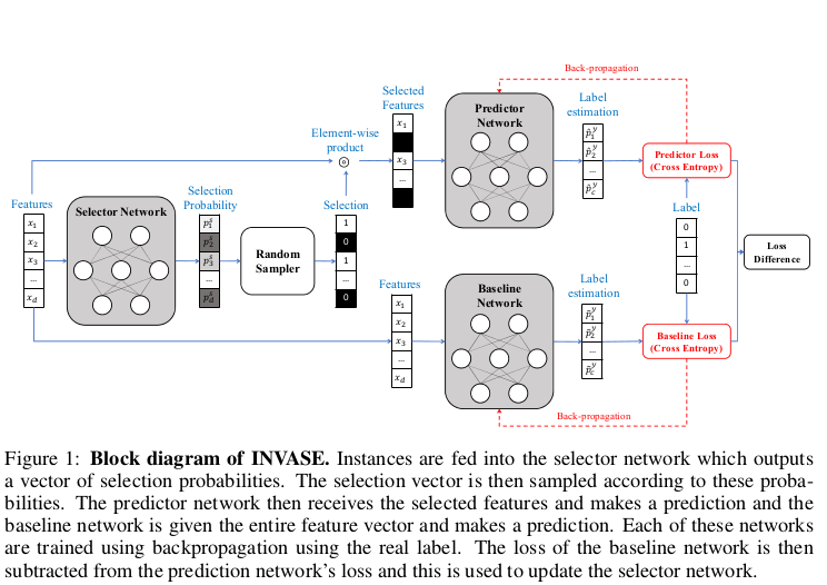
\[\begin{aligned} l(\theta) &=\mathbb{E}_{(\mathbf{x}, y) \sim p}\left[\mathbb{E}_{\mathbf{s} \sim \pi_{\theta}(\mathbf{x}, \cdot)}\left[\hat{l}(\mathbf{x}, \mathbf{s})+\lambda\|\mathbf{s}\|_{0}\right]\right] \\ &=\int_{\mathcal{X} \times \mathcal{Y}} p(\mathbf{x}, y)\left(\sum_{\mathbf{s} \in\{0,1\}^{d}} \pi_{\theta}(\mathbf{x}, \mathbf{s})\left(\hat{l}(\mathbf{x}, \mathbf{s})+\lambda\|\mathbf{s}\|_{0}\right)\right) d x d y \end{aligned}\]To get more clarity into how the different pieces fit together, have a look at the block diagram at the start of this section.
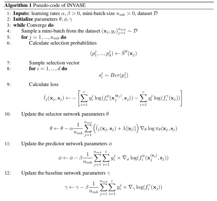
The psuedocode for the INVASE alogrithm is given below where we can see that the three networks(selector, predictor and baseline) are trained iteratively untill convergence.
 Taken from the INVASE[1] paper
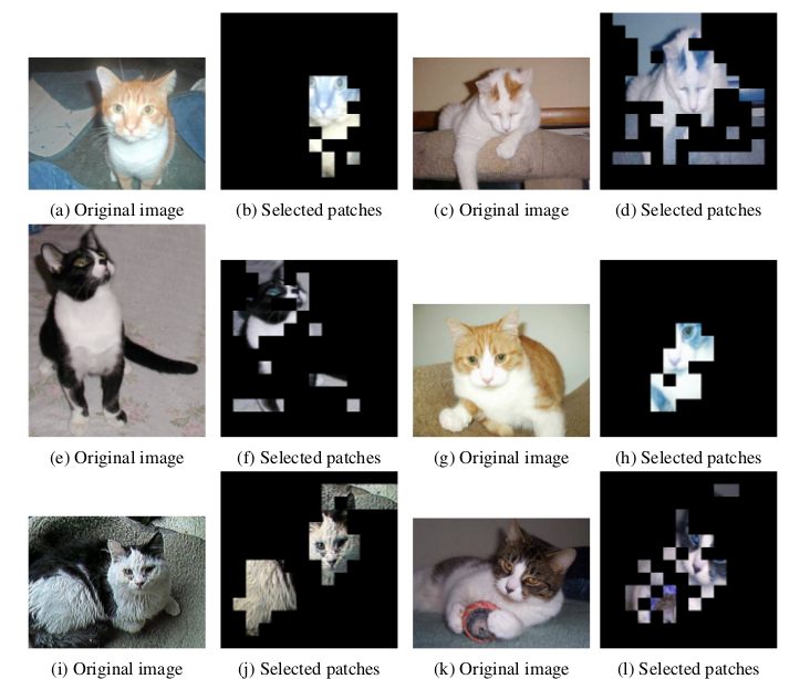
Results
For the sake of nice visualization, I have shown below the results of INVASE for computer vision i.e. classification on Kaggle Dogs vs. Cats dataset.
 Taken from the INVASE[1] paper
References
- Yoon J, Jordon J, van der Schaar M. INVASE: Instance-wise variable selection using neural networks. InInternational Conference on Learning Representations 2018 Sep 27.
- Chen J, Song L, Wainwright M, Jordan M. Learning to explain: An information-theoretic perspective on model interpretation. InInternational Conference on Machine Learning 2018 Jul 3 (pp. 883-892). PMLR.